 |
| EA3IW WSPR on 475 kHz with 200 milliwatt with a 4 x 15 meter loop |
Posts tonen met het label WSPR Analysis. Alle posts tonen
Posts tonen met het label WSPR Analysis. Alle posts tonen
woensdag 17 januari 2018
Daily changes in propagation on 472 kHz
WSPR reveals the daily changes in propagation. It is not a surprise to see that in the 472 kHz band most spots are made during the night. As you can see most spots are made in the hour of 23 UTC and 00 UTC.
Click on the table to enlarge.
maandag 15 januari 2018
EA3IW WSPR on 472 kHz with 200 milliwatt

Calculations show that the radiated power is about 200 milliwatt.
The spots were made from 26th of December 2017 till the 6th of January 2018.
To reduce the length of the table, I only show the data of the receiving stations, that reported during all of the days that are shown in the table.
The lower the calculated lowest possible power, the better the propagation. The columns at the right show the spots with the strongest signal. (10 dB over 3 columns)
 |
| EA3IW WSPR on 475 kHz with 200 milliwatt from a 4 x 15 meter loop |
In the table the stations are sorted by distance.
The column of 200 mW shows the spots that were just strong enough to be decoded. The column of 20 mW and 2 mW show the spots that were 10 dB stronger and 20 dB stronger. The lower the Lowest possible power the stronger the signal.
EA3IW-3 is a receiver at a distance of 100 km of the transmitter of Albert. The table shows that in 130 spots the full power of 200 mW was needed to be heard. 205 Spots could have been made with 100 mW and 5 spots even be received if they were made with 20 mW.
The spots of EA2HB show a dynamic range of 16 dB, from 5 mW to 200 mW.
The most sensitive station is F6GEX. The one spots with the strongest signal, could have been made with 0.5 mW. Notice that 262 out of 1126 spots, received by F6GEX, could have been made with 5 mW. The difference between the spots with 200 mW and the strongest spot (0.5 mW) is 26 dB.
The results show that it is possible to use WSPR with a low power even on 475 kHz.
The changes in propagation are best seen, when you run WSPR 24 hours a day.
Thanks to Albert, for the interesting low power results and the pictures that I received.
Click to discover how to calculate the Calculated lowest possible power.
zondag 12 maart 2017
G4EFE WSPR with 5 mW on 40 m
Martin G4EFE is an enthusiast milliwatt WSPRer.
I curiously follow the WSPR adventures of Martin in which he uses very low power.
Here I show new analysis of the spots that Martin made with a power of 5 milliwatt on 40 m with a full-size 40 m square loop.
The table shows the number of spots over a three day period, from day to day and hour to hour.
From the used power of 5 mW (in all spots) and the SNR, I calculated the lowest possible power.
A spot with a SNR of -28 dB is a "solid copy" in WSPR. So when, for instance, the SNR is -18 dB, the signal is 10 dB stronger and could have been 10 dB lower and still give a solid copy, with a SNR of -28 dB.
Propagation
In the spots that were received by F6EHP, you can see the development of the propagation from hour to hour. You can see that the signal peaks at 9 UTC at 3-2-2017. The strongest spot could be made with a power of 0.1 milliwatt. This is also the strongest spot in this table.

Martin uses his IC703 and an attenuator to make a power of 5 milliwatt. His antenna is a full-size 40 m square loop. As I saw on WSPRnet.
I curiously follow the WSPR adventures of Martin in which he uses very low power.
Here I show new analysis of the spots that Martin made with a power of 5 milliwatt on 40 m with a full-size 40 m square loop.
The table shows the number of spots over a three day period, from day to day and hour to hour.
From the used power of 5 mW (in all spots) and the SNR, I calculated the lowest possible power.
A spot with a SNR of -28 dB is a "solid copy" in WSPR. So when, for instance, the SNR is -18 dB, the signal is 10 dB stronger and could have been 10 dB lower and still give a solid copy, with a SNR of -28 dB.
The better the SNR, the stronger the signal and the
lower the calculated lowest possible power will be.
lower the calculated lowest possible power will be.
In the spots that were received by F6EHP, you can see the development of the propagation from hour to hour. You can see that the signal peaks at 9 UTC at 3-2-2017. The strongest spot could be made with a power of 0.1 milliwatt. This is also the strongest spot in this table.
Martin uses his IC703 and an attenuator to make a power of 5 milliwatt. His antenna is a full-size 40 m square loop. As I saw on WSPRnet.
donderdag 9 februari 2017
G4EFE WSPR with 5 mW on 40 m
WSPR is a beacon system that is designed for low power. How low can you go?
Martin G4EFE ran WSPR with very low power.
Martin G4EFE wrote after experimenting with 1 mW, using his attenuator of and 20 dB:
So I've had a little time for some experimentation, and the results - I think - are spectacular. Attenuating the output to just 1mW netted me several spots from neighboring countries.
Best DX was GM* at 711km, who reports me at -18b dB SNR, suggesting I can go even lower.
So today I'm running just 100 MICROWATTS. I can't believe anyone will spot me, but I'm the optimistic kind! Thanks again, Bert, for this easy and fun station accessory.
The map, the tabel for 1mW and the picture of the beautiful attenuator can be found here: https://www.flickr.com/photos/71155570@N00/albums/72157679958156316
OK Martin, thank you for sharing this fine info.
5 mW down to 1 mW
Martin started with 5 milliwatt for three days, as you can see in both tables. On the 5th the power was reduced to 2 milliwatt. On the 6th Martin had great fun in 21 spots with just 1 milliwatt.
To make a power of 1 milliwatt Martin uses his IC703, at it's lowest setting with 100 mW and an attenuator of 20 dB. His antenna is a full-size 40 m square loop. As I saw on WSPRnet.
From hour to hour
In the table below you can see the number of spots in each hour.
The days go from the bottom to the top.
The number of spots vary from day to day. this is not only propagation.
Martin is constantly transmitting, but the listeners can be jumping from band to band.
The best DX from GM*with a SNR of -18 dB, that Martin refers to, gives a calculated lowest possible power of 0.1 milliwatt. This spot could be made with 0.1 mW and still be a solid copy with a SNR of -28 dB. See the spot in the red circle in the table below.
The better the propagation, the better the SNR will be and the lower the Calculated lowest possible power. The Calculated lowest possible power is calculated from the power and the SNR.
Martin G4EFE ran WSPR with very low power.
Martin G4EFE wrote after experimenting with 1 mW, using his attenuator of and 20 dB:
So I've had a little time for some experimentation, and the results - I think - are spectacular. Attenuating the output to just 1mW netted me several spots from neighboring countries.
Best DX was GM* at 711km, who reports me at -18b dB SNR, suggesting I can go even lower.
So today I'm running just 100 MICROWATTS. I can't believe anyone will spot me, but I'm the optimistic kind! Thanks again, Bert, for this easy and fun station accessory.
The map, the tabel for 1mW and the picture of the beautiful attenuator can be found here: https://www.flickr.com/photos/71155570@N00/albums/72157679958156316
OK Martin, thank you for sharing this fine info.
5 mW down to 1 mW
Martin started with 5 milliwatt for three days, as you can see in both tables. On the 5th the power was reduced to 2 milliwatt. On the 6th Martin had great fun in 21 spots with just 1 milliwatt.
To make a power of 1 milliwatt Martin uses his IC703, at it's lowest setting with 100 mW and an attenuator of 20 dB. His antenna is a full-size 40 m square loop. As I saw on WSPRnet.
From hour to hour
In the table below you can see the number of spots in each hour.
The days go from the bottom to the top.
The number of spots vary from day to day. this is not only propagation.
Martin is constantly transmitting, but the listeners can be jumping from band to band.
 |
| G4EFE WSPR with 5 mW down to 1 mW - From hour to hour |
 |
| G4EFE WSPR with 5 mW to 1 mW, using an attenuator |
dinsdag 17 november 2015
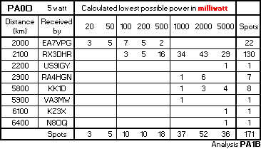
PA0O with WSPR on 160 m
Here is an analysis of very interesting WSPR spots, that were made by Jaap PA0O. The spots were made from the 19th of oktober until the 12th of november 2015. The band was 160 meter. To reduce the length of the table, I only listed the stations that received more than 60 spots.
The strongest signal was received by G8DYK over a distance of 600 km. The longest distance was 6400 km, to N8OQ.

A Calculated lowest possible power of 1 milliwatt, means that a signal with a power of 1 milliwatt, should be received with a SNR of -29 dB. This is a solid copy in WSPR.
Spots over 2000 km or more.
zondag 7 juni 2015
Solar Eclipse WPA of WSPR spots by PE4BAS
Solar Eclipse WSPR Propagation Analysis (WPA) of spots by PE4BAS.
The spots were made on 160 mtr, during daylight hours.
The lower the Lowest Possible Power, the better the propagation.

The spots were made on 160 mtr, during daylight hours.
The lower the Lowest Possible Power, the better the propagation.
zaterdag 2 mei 2015
6 m WSPR analysis for Roger G3XBM
In his informative Blog, Roger G3XBM wrote about aircraft scattering of signals on 6 m.
I had the pleasure of making an analysis of the WSPR spots reported by Roger.
Drift
In WSPR the drift is measured over a period of 1 minute, so the drift is given in Hz per minute.
Recently I included Drift in my Excel spread sheet that I use to make an analysis.
Analysis

A few day ago I wrote to Roger: See article
Hello Roger,
This evening I took some time to make an analysis of a number of spots on 6 meter.
I took the most interesting spots for airplane scatter.
I hope you like it and can place it in your blog.
I left in M0EMM to show the difference. hi
Positive drift means the path is becoming shorter.
The spots of M0MVB shows spots where the path is becoming shorter (+3Hz per minute)
and spots where the path is becoming longer. (-2 Hz per minute)
I just saw that the spots of M0YOU with scatter, are much stronger than the spot without scatter.
The lower the lowest possible power, the stronger the signal.
A lowest possible power of 1 mW is 17 dB stronger than 50 mW. hi.
I left in the spots of M0EMM, to show that there is no Doppler and the signals are not that strong.
Good luck in further analysis,
73, Bert PA1B
I had the pleasure of making an analysis of the WSPR spots reported by Roger.
Drift
In WSPR the drift is measured over a period of 1 minute, so the drift is given in Hz per minute.
Recently I included Drift in my Excel spread sheet that I use to make an analysis.
Analysis
- The value in the table, such as -4, is a spot with a drift of -4 Hz per minute.
Positive drift means that the radio path is getting shorter and negative is longer. - The signals of M0MVB show spots with a drift of -2 and 3 Hz per minute.
It is possible, that there is a flight paths involved in the spots with -2 and an other path with the spots of 3 Hz per minute. - The scattered signals with drift, sent by M0YOU are very strong, with a lowest possible power of 1 mW. The spot with no drift (0 Hz per minute) has a lowest possible power of 50 mW, thus is 17 dB weaker.
- The signals of M0EMM show no drift. So it's possible that there is no airplane scatter here, but an other form of propagation, such as difraction. Notice that all these spots are made within one hour.
Thanks to Roger. FB.
A few day ago I wrote to Roger: See article
Hello Roger,
This evening I took some time to make an analysis of a number of spots on 6 meter.
I took the most interesting spots for airplane scatter.
I hope you like it and can place it in your blog.
I left in M0EMM to show the difference. hi
Positive drift means the path is becoming shorter.
The spots of M0MVB shows spots where the path is becoming shorter (+3Hz per minute)
and spots where the path is becoming longer. (-2 Hz per minute)
I just saw that the spots of M0YOU with scatter, are much stronger than the spot without scatter.
The lower the lowest possible power, the stronger the signal.
A lowest possible power of 1 mW is 17 dB stronger than 50 mW. hi.
I left in the spots of M0EMM, to show that there is no Doppler and the signals are not that strong.
Good luck in further analysis,
73, Bert PA1B
zondag 5 april 2015
Lowest possible power
In WSPR analyses I use the lowest possible power to compare the signal strength of WSPR spots.
The lowest possible power is calculated from the transmitted power and the SNR of the receiving station. The lowest possible power is an excellent propagation indicator.
Click on the Tab: WSPR propagation analysis at the top of the Blog for a new explanation on the lowest possible power and a easy to use beatiful table.
I am proud at the beautiful table. hi.
The lowest possible power is calculated from the transmitted power and the SNR of the receiving station. The lowest possible power is an excellent propagation indicator.
Click on the Tab: WSPR propagation analysis at the top of the Blog for a new explanation on the lowest possible power and a easy to use beatiful table.
 |
| Lowest possible power - Click to enlarge PA1B |
zaterdag 28 maart 2015
K5MQ WSPR 100mW on 40 Meters (2)
Dave K5MQ has been running WSPR for 4 days at 100 mW output on 40 meters.
To show the behavior of the propagation from day to day, I made a overview for four days.
Horizontally you find the time in UTC in blocks of 1 hour.
Each rectangular black block indicates an hour, in which one or more spots occurred and the calculated lowest possible power of that spot(s).
Vertically you find the lowest possible power, which is a good indication of the signal strength.
The lowest possible power is calculated from the power of the sending station and the SNR of the receiving station. The higher the SNR, the better the propagation and the lower the lowest possible power.
Please notice, that not all patterns in this propagation diagram,
can be easily recognized and can be easily explained. hi.
Propagation to WB5WPA over 500 km
Dave 's signal was received by WB5WPA over a distance of 500 km at 13 utc on the 24th with a calculated lowest possible power of 1 milliwatt.
From 13 utc on the signal becomes weaker. At 18 utc the signal is 10 dB weaker.
From18 utc to 1 utc on the next day, the process is reversed.
At 1 utc the signal has the same signal strength as at 12 utc of the previous day.
Propagation to N8SDR over 1100 km
On the 24th we see the same pattern in the propagation, but this time throughout the night, between 3 utc and 10 utc. At 3 utc the signal suddenly appears and is immediately very strong . Than rapidly becomes weaker (16 dB) and than gradually becomes stronger again, to reach the highest value at 10 utc.
Electrical field strength
Dave noticed that K9AN at a distance of 1003 km copied his 100 mW throughout the daylight hours, many times. And that he must have a great receiver there.
To compare the signals of the different stations I made an analysis of the received signals by the Electrical field strength in micro Volt per meter.
The analysis below shows that K9AN, N8SDR and KE7TYT received Dave's signal with the same field strength. hi. The difference between each of the columns is 5 dB.

A calculated lowest possible power of 1 milliwatt means that a signal of 1 mW,
could be received with a SNR of -29 dB.
To show the behavior of the propagation from day to day, I made a overview for four days.
This analysis uses the same data as Blog entry of yesterday, but also shows the relative signal strength of the received signal.
Each rectangular black block indicates an hour, in which one or more spots occurred and the calculated lowest possible power of that spot(s).
Vertically you find the lowest possible power, which is a good indication of the signal strength.
The lowest possible power is calculated from the power of the sending station and the SNR of the receiving station. The higher the SNR, the better the propagation and the lower the lowest possible power.
The lower the lowest possible power, the better the propagation.
Please notice, that not all patterns in this propagation diagram,
can be easily recognized and can be easily explained. hi.
 |
| Propagation diagram. K5MQ WSPR on 40 m with 100 mW. |
Dave 's signal was received by WB5WPA over a distance of 500 km at 13 utc on the 24th with a calculated lowest possible power of 1 milliwatt.
From 13 utc on the signal becomes weaker. At 18 utc the signal is 10 dB weaker.
From18 utc to 1 utc on the next day, the process is reversed.
At 1 utc the signal has the same signal strength as at 12 utc of the previous day.
For the distance of 500 km we can see, that when the signal is reflected
in the ionosphere, the propagation is immediately at it's best.
in the ionosphere, the propagation is immediately at it's best.
From that moment, the signal will be weaker, until the process is reversed.
Propagation to N8SDR over 1100 km
On the 24th we see the same pattern in the propagation, but this time throughout the night, between 3 utc and 10 utc. At 3 utc the signal suddenly appears and is immediately very strong . Than rapidly becomes weaker (16 dB) and than gradually becomes stronger again, to reach the highest value at 10 utc.
Electrical field strength
Dave noticed that K9AN at a distance of 1003 km copied his 100 mW throughout the daylight hours, many times. And that he must have a great receiver there.
To compare the signals of the different stations I made an analysis of the received signals by the Electrical field strength in micro Volt per meter.
The analysis below shows that K9AN, N8SDR and KE7TYT received Dave's signal with the same field strength. hi. The difference between each of the columns is 5 dB.
A calculated lowest possible power of 1 milliwatt means that a signal of 1 mW,
could be received with a SNR of -29 dB.
vrijdag 27 maart 2015
K5MQ WSPR 100mW on 40 Meters
Dave K5MQ reports on his blog, that he has been running WSPR for 4 days at 100 mW output on 40 meters. He wanted to try lower power on 40 meters, than he did on 160 m.
The analysis shows the stations, that spotted Dave for 3 days or more.
Under UTC you find the number of spots from hour to hour.
E.g. K9AN was spotted 3 times on 2015-03-22 between 23:00 and 23:59 UTC
Futher, I also chose to show two stations with the largest distance.
KL7L from Alaska and EA/LA3JJ from Spain.
 |
| WSPR spots of Dave K5MQ on 40 m with 100 mW |
zaterdag 28 februari 2015
K5MQ WSPRs on 1.8 MHz with 1 W
I received a fine comment from Dave K5MQ on my previous post:
Dave further mentioned that he was using WSPR with a power of 1 W om 160 m.
Dave wrote:
I usually run WSPR with 1 watt here.
Have been on 160 meter WSPR the last few days.
Have received a 3 stations from the UK, two at 5w and one at 20w.
The furthest my 1 watt has been heard is VE6 at 2994km from my QTH in Lousiana.
Using a full size dipole for 160m.
73, Dave K5MQ
Here is a table with spots from Daves 1W WSPR signal from the 16th to the 28th of February 2015.
The lower the Calculated Lowest possible power, the better the propagation.
 How to read the table:
K9AN at a distance of 1000 kilometer, received Daves signal 143 times.
45 Of these spots were received with a SNR of about -9 dB.
So the Calculated Lowest possible power is 10 mW
The lower the Calculated Lowest possible power, the better the propagation.
Thanks to Dave K5MQ.
It's my pleasure to make the WPA (WSPR propagation analysis)
Visit Dave's Blog entry on WSPR on 160 meters.
* The Calculated lowest possible power is the power that could by received with a SNR of -29 dB.
The stronger the signal the lower the Calculated lowest possible power.
A signal with a SNR of -29 dB is a solid copy in WSPR.
Dave further mentioned that he was using WSPR with a power of 1 W om 160 m.
Dave wrote:
I usually run WSPR with 1 watt here.
Have been on 160 meter WSPR the last few days.
Have received a 3 stations from the UK, two at 5w and one at 20w.
The furthest my 1 watt has been heard is VE6 at 2994km from my QTH in Lousiana.
Using a full size dipole for 160m.
73, Dave K5MQ
Here is a table with spots from Daves 1W WSPR signal from the 16th to the 28th of February 2015.
The lower the Calculated Lowest possible power, the better the propagation.
K9AN at a distance of 1000 kilometer, received Daves signal 143 times.
45 Of these spots were received with a SNR of about -9 dB.
So the Calculated Lowest possible power is 10 mW
The lower the Calculated Lowest possible power, the better the propagation.
Thanks to Dave K5MQ.
It's my pleasure to make the WPA (WSPR propagation analysis)
Visit Dave's Blog entry on WSPR on 160 meters.
* The Calculated lowest possible power is the power that could by received with a SNR of -29 dB.
The stronger the signal the lower the Calculated lowest possible power.
A signal with a SNR of -29 dB is a solid copy in WSPR.
donderdag 26 februari 2015
WSPR with 5 watts
 From time to time I visit the WSPR database to look for interesting spots that are made with very low power.
But this time I was wondering, if there are many operators, that use much more than 5 watts.
To my surprise only a few operators used 10 to 1000 watts.

The WSPR spots are collected on 10 meters in 24 hours.
I chose 24 hours to include all operators, that skip from band to band, following the changes in propagation, in all the parts of the world.
The interval lasted from 9:02 utc on the 20th of February to 9:00 utc on the 21st.
I selected the 10 meter band, because in the days before, I made an analysis of spots on 10 meters.
Power categories
The table shows the number of spots that were made in each power category from
1 mW to 5000 mW (5 W) (QRP)
and the number of spots that were made with 10 to 1000 watts.
Results
In the power categories from 1 milliwatt to 5 watts, most spots were made in the category of 5 watts.
This is 42 % of all spots.
I am pleased to see that many operators use 200 mW* or 500 mW.
200 mW in 15% of all spots and 500 mW in 16% of all spots.
It's good to see that only a few operators use 10 W to 1000 W. (See also "one kW")
One kW
Not all spots that show up in the database with 1000 W, are actually made with 1000 W.
In the past I have seen WSPR spots from an operator that used a homebrew QRP rig, that he proudly showed on QRZ. But the setting in his WSPR program was wrong. He discovered the mistake.
Later the spots showed a power of 2 watts in stead of 1000 watts. hi.
* Did you know that 200 mW in WSPR can be compared with 4 Watts in CW and 80 Watts in SSB.
So with 200 mW in WSPR you can see where you 4 watt CW signal could be heard. hi.
zaterdag 3 januari 2015
WSPR Propagation Analysis - G3XBM 28 MHz Dec 2014 (2)
The propagation changes from day to day, as you can read in the blog of Roger G3XBM.
Here is an analysis of the WSPR spots of G3XBM that were received by K9AN
on the 24th and the 28th of December 2014.
The time is given in UTC.
on the 24th and the 28th of December 2014.
The time is given in UTC.
The diagrams show a lot of spots, since K9AN listens every two minutes. hi
The lower the calculated lowest possible power, the better the propagation.
On the 24th, the propagation is at it's best around 13:50 UTC and 17:06 UTC,with a calculated lowest possible power of 5 milliwatts.
 |
| Click to enlarge. G3XBM received by K9AN on 2014-12-24 |
On the 28th the propagation has a short peak at 14:52 UTC.
Around that time there are seven successive spots, every two minutes.
In the spot of 16:36 utc, the full power of 500 mW is needed, to be spot. hi.
 |
| G3XBM received by K9AN on 2014-12-28 |
In most of the spots, the calculated lowest possible power is 50 mW or less, on both days.
This means that, if you would use CW instead of WSPR, that 1 watt (20 * 50 mW) could be used to make QSO's in CW.
vrijdag 2 januari 2015
WSPR Propagation Analysis - G3XBM 28 MHz Dec 2014
Roger G3XBM ran his WSPR signal for several days on 28 MHz.
This provides interesting information on propagation on 28 MHz.
I collected data from the WSPR database, to make the diagrams.
The first two diagrams, show spots that are collected over several days.
The strongest spots are given in red.

The first two diagrams show the calculated electrical field strength in micro volt per meter.
If spots show the same field strength, the voltage on the antenna will be the same, for a simple wire antenna.
The difference between the successive values of the field strength is 5 dB.
This is about one S-point, since 6 dB is one S-point.
The lower the value, the better the propagation.
So 0.03 micro volt/meter is about 1 S-point stronger than 0.06 micro volt/meter.

The strongest spot over 900 km was 2 S-points down, compared to the spot over 5300 km

Notice that the spots over 5300, 6500 and 14700 km were made with the same field strength at the receiving antenna, so the strength of the signal that arrived on the antenna was the same in these three spots.
Further analysis shows which receiving stations have Excellent Ears. See the spots in red.
The spots in red in the table below correspond to the spots in red in the tables above.
Power in CW
I was wondering, how much power would be needed to make CW QSO's.
For a CW QSO you need twenty times more power, (Click) than for a WSPR spot. (13 dB)
The diagram below shows the Calculated lowest possible power (Click)in milliwatt for each spot.
 For the strongest WSPR signal, received by K9AN the calculated lowest possible power is 2 mW.
Thsi means that the that 2 mW would be received with a SNR of -29 dB. (Solid copy in WSPR)
To be received in CW, a power of 20 * 2 = 40 mW would be needed.
This does not surprise me a bit, since I made a CW contest QSO with K3WW on 21 MHz in 2012 with 36 mW.
Rogers signal was also heard in VK. The calculated lowest possible power was 5 mW.
So in CW his signal would be heard with 20 * 5 = 100 mW.
This seem too low, but please notice that to double the distance it takes an increase of 1 S-point (6 dB) to get the same field strength.
One S-point means four times more power.
Further, please notice that WSPR is patient and tireless.
It is even possible that one of the operators was a sleep during the time that the spot was made. hi.
This provides interesting information on propagation on 28 MHz.
I collected data from the WSPR database, to make the diagrams.
The first two diagrams, show spots that are collected over several days.
The strongest spots are given in red.

The first two diagrams show the calculated electrical field strength in micro volt per meter.
If spots show the same field strength, the voltage on the antenna will be the same, for a simple wire antenna.
The difference between the successive values of the field strength is 5 dB.
This is about one S-point, since 6 dB is one S-point.
The lower the value, the better the propagation.
So 0.03 micro volt/meter is about 1 S-point stronger than 0.06 micro volt/meter.
The strongest (in red) spots show the same field strength.
Notice that the spots over 5300, 6500 and 14700 km were made with the same field strength at the receiving antenna, so the strength of the signal that arrived on the antenna was the same in these three spots.
Further analysis shows which receiving stations have Excellent Ears. See the spots in red.
The spots in red in the table below correspond to the spots in red in the tables above.
 |
| The stations with excellent ears. |
I was wondering, how much power would be needed to make CW QSO's.
For a CW QSO you need twenty times more power, (Click) than for a WSPR spot. (13 dB)
The diagram below shows the Calculated lowest possible power (Click)in milliwatt for each spot.
Thsi means that the that 2 mW would be received with a SNR of -29 dB. (Solid copy in WSPR)
To be received in CW, a power of 20 * 2 = 40 mW would be needed.
This does not surprise me a bit, since I made a CW contest QSO with K3WW on 21 MHz in 2012 with 36 mW.
Rogers signal was also heard in VK. The calculated lowest possible power was 5 mW.
So in CW his signal would be heard with 20 * 5 = 100 mW.
This seem too low, but please notice that to double the distance it takes an increase of 1 S-point (6 dB) to get the same field strength.
One S-point means four times more power.
Further, please notice that WSPR is patient and tireless.
It is even possible that one of the operators was a sleep during the time that the spot was made. hi.
zaterdag 8 november 2014
10m WSPR - 5 watts from M0DEV
Mark M0DEV uses WSPR with 5 watts.
.png)
.png)
.png)
Today he made more than 400 spots on 10 m.
I noticed this since Mark left a note on the Blog of Roger G3XBM.
Mark notes:
Interesting. I am running 5 W (it's as low as my rig will go) and our two 3 hourly plots on wspr are all but identical. Neither of us has made any headway with the west side of the states.
The conclusion I draw is that when the band is open, it's open, and when it is shut it is shut:
The conclusion I draw is that when the band is open, it's open, and when it is shut it is shut:
there is no point trying to blast it open with QRO.
The analysis below shows the calculated lowest possible power.
The lowest possible power is calculated from the power sent and the SNR.
The better the SNR, the lower the lowest possible power, the better the propagation.
The analysis shows that the propagation was good this day and confirms Marks statement that QRO is not needed.
Please notice that even with 100 mW, Marks signal would be heard over a large distance.
Please notice that even with 100 mW, Marks signal would be heard over a large distance.
vrijdag 26 september 2014
WSPR Propagation Analysis - G3XBM 28 MHz
Many WSPR operators jump from one band to the next, when band conditions changes.
Roger G3XBM ran his WSPR signal for several days on 28 MHz.
This provides interesting information on propagation on 28 MHz.
I collected data from the WSPR database, to make this diagram.
.png)
Roger G3XBM ran his WSPR signal for several days on 28 MHz.
This provides interesting information on propagation on 28 MHz.
I collected data from the WSPR database, to make this diagram.
In this diagram, I choose to show the spots of Roger received by DK6UG over 600 kilometer and LB9YE over 1500 km.
The diagram shows the number of spots for a day and from hour to hour.
The stronger the signal, the lower the calculated lowest possible power.
DK6UG over 600 km
It's interesting to see that the propagation to DK6UG changes from day to day.
On the 13th there are two peaks in the propagation, with no propagation in between.
On the 14th there is only a spot on 18 UTC.
This is at the same time of the peak of the day before.
On the 15th there are 3 peaks at 11, 14 and 19 UTC
The 17th is the most interesting day.
The day starts with reception on 11 till 12:58 UTC.
The 17th shows one very strong spot at 14:10 UTC with a calculated lowest possible power of 10 mW. The next spot with a CLPP of 1000 mW was on 14:54 UTC. Notice that in this spot the signal strenght is 20 dB lower.
Please notice that there is no reception from 13:00 till 13:58 UTC on all days,except for the 19th.
LB9YE over 1500 km versus DK6UG over 600 km
Most interesting are 13th and 14th
At the 13th the propagation is good to DK6UG, but not to LB9YE.
At the 14th it's the other way around.
Most interesting are 13th and 14th
At the 13th the propagation is good to DK6UG, but not to LB9YE.
At the 14th it's the other way around.
vrijdag 12 september 2014
PC4T with 5 watts on 14 MHz with WSPR
In addition to the update of the post of 2014-09-08, I made a new analysis of the spots between made over a distance 1500 km to 2200 km.
The spots were made during the morning.

The spots were made during the morning.
maandag 8 september 2014
PC4T with 5 watts on 14 MHz with WSPR
Here is a WSPR Propagation Analysis of spots of Paul PC4T on 14 MHz.
The lower the Calculated lowest possible power, the better the propagation.
Nearly all spots over 1100 to 2200 kilometer could have been made with 20 milliwatts.

Update 2014-09-10
I made an extra analysis of the spots in the red fields.
The spots were made from 19:12 till 19:40 UTC
The lower the Calculated Lowest Possible Power, the better is the propagation.

The lower the Calculated lowest possible power, the better the propagation.
Nearly all spots over 1100 to 2200 kilometer could have been made with 20 milliwatts.
Update 2014-09-10
I made an extra analysis of the spots in the red fields.
The spots were made from 19:12 till 19:40 UTC
The lower the Calculated Lowest Possible Power, the better is the propagation.
LA9JO at 2000 km
The signal strength increases with 6 dB (in power 4x as strong) from 19:12 till 19:40 utc.
SV8QG
The last spot is 14 dB weaker than the first.
VK5MR
The last spot is slightly stornger than the other two.
donderdag 8 mei 2014
G4ILO Whispering with 20 mW and 1 mW
 This is an other analysis of the data collected from the
 WSPR database for spots of Julian G4ILO.
Julian transmitted with a power of 1 mW and 20 mW.
The table shows, that the spots that were made with 1 mW,
were about 10 dB weaker than the spots made with 20 mW
The table shows a selection stations that received spots made with both 20 mW and 1 mW
To compare spots over different distances, I use the
Calculated electrical field strength, E, in microVolt per meter.
For details see the WSPR Propagation Analysis page of this Blog.
The lower the electrical field strength the better the propagation.
A power ratio of 10 means 10 dB.
Please notice the the value for E is given in Volt/m, so a Voltage ratio of 10 means 20 dB.
Which is indicated at the top of the table.
A Voltage ratio of 10 is a ratio of 100 in power.
The table shows stations that received the signals, that were transmitted with 1 mW and 20 mW.
Notice the difference in field strength in spots made with 1 mW or 20 mW.
The difference in field strength between the spots of 1 mW and 20 mW is about two steps in this table.
This is about 10 dB.
This is about 10 dB.
This is no surprise because, the difference in power between 1 mW and 20 mW
is 10 log (20 / 1) = 13 dB.
The differences in propagation are huge.
The field strength of the spots made with 20 mW, received by ON7KO over 600 km,
show a value of 0,3 microV/m to 0,03 microVolt/m.
The ratio in voltage is 10 and the ratio in power is 100, which is 20 dB. Wow.

vrijdag 11 april 2014
"WSPR Propagation Analysis" for WSPR spots of G3XBM on 10 m
Roger, G3XBM wrote:
Nothing at all was seen until mid-afternoon and then the band just opened wide!
K9AN (6505km) last spotted my 2W signal at 2308z, which is after midnight local time and HOURS after the band has normally died out. It had been dark for hours. One wonders if this was F2 or even multi-hop Es? I wonder what was happening on 6m transatlantic? I must check.
(Spots made on 2014-04-08) Click to visit the article.
I was interested, so I made an WSPR Propagation Analysis of the spots on that day and the days before. The second table shows the last spot at 23:08 UTC, but also reveals the rapid change in propagation around 22:20 UTC.


How to read the table
In the analysis above, I show the "Calculated Lowest possible Power" in milliwatt and the hours of the day in UTC. The lower the "Calculated Lowest Possible Power", the better the propagation.
Roger is refering to WSPR spots made on 2014-04-08.
At the bottom of the table above.
From 10 UTC to 22 UTC the propagation gets better.
The best propagation occurred in the spot with the red star made on 22:20 UTC.
Even more spectacular
The best propagation on 2014-03-28, at the top of the table, occurred between 13:00 and 15:59 UTC in the aftenoon.
But even more spectacular is the change in propagation in the 3 spots * that were made between 22:00 and 22:22 UTC, that show a very rapid chang in propagation. (See the red arrows)
Thanks to Roger for the interesting experiments with WSPR.
Nothing at all was seen until mid-afternoon and then the band just opened wide!
K9AN (6505km) last spotted my 2W signal at 2308z, which is after midnight local time and HOURS after the band has normally died out. It had been dark for hours. One wonders if this was F2 or even multi-hop Es? I wonder what was happening on 6m transatlantic? I must check.
(Spots made on 2014-04-08) Click to visit the article.
I was interested, so I made an WSPR Propagation Analysis of the spots on that day and the days before. The second table shows the last spot at 23:08 UTC, but also reveals the rapid change in propagation around 22:20 UTC.
How to read the table
In the analysis above, I show the "Calculated Lowest possible Power" in milliwatt and the hours of the day in UTC. The lower the "Calculated Lowest Possible Power", the better the propagation.
To compare the propagation over several days,
I included 2014-03-28 till 2014-04-08.Roger is refering to WSPR spots made on 2014-04-08.
At the bottom of the table above.
From 10 UTC to 22 UTC the propagation gets better.
The best propagation occurred in the spot with the red star made on 22:20 UTC.
Even more spectacular
The best propagation on 2014-03-28, at the top of the table, occurred between 13:00 and 15:59 UTC in the aftenoon.
But even more spectacular is the change in propagation in the 3 spots * that were made between 22:00 and 22:22 UTC, that show a very rapid chang in propagation. (See the red arrows)
Thanks to Roger for the interesting experiments with WSPR.
Abonneren op:
Posts (Atom)